Worked examples — Linear Quadratic Regulator (LQR) — Riccati equation, optimal gains

Before we start, we rebuild — from the general Riccati equation, right here on this page — the scalar formula we lean on repeatedly, so nothing below depends on remembering the parent note.

---

The scenario matrix

Every LQR problem lives in one of these cells. Each column is a knob; each row is a value that knob can take. The worked examples below each stamp which cell(s) they land in.

Cell	Plant sign / structure	Weight regime	What it stress-tests
A	Scalar, stable ($a<0$)	balanced $q=r$	baseline, positive root
B	Scalar, unstable ($a>0$)	balanced	control must create stability
C	Scalar, marginal ($a=0$)	balanced	the integrator edge case
D	Scalar	cheap control $r\to 0$	limiting: gain blows up
E	Scalar	expensive control $r\to \infty$	limiting: gain fades, must rely on plant
F	2-state double integrator	vary $\rho$	LQR = PD, pole placement
G	2-state	$Q$ degenerate (rank-deficient)	observability of $\sqrt{Q}$ needed
H	Any	$Q\to$ huge vs $R$	aggressiveness / ratio-only rule
I	Uncontrollable plant	any	recipe fails — must recognize it
J	Word problem (satellite)	design task	pick $\rho$ for a spec

We now cover A–J.

---

Worked examples

Example 1 — Cell A: stable scalar plant, balanced weights

Forecast: the plant is already stable ($a=-2<0$). Do you think LQR still pulls the pole further left, or leaves it alone? Guess before reading.

1. Write the scalar Riccati. $2ap-\frac{b^2}{r}{p}^2+q=0\Rightarrow -4p-p^2+1=0.$ Why this step? We derived $2ap-\frac{b^2}{r}{p}^2+q=0$ in the box above; we just substituted $a=-2,b=1,q=1,r=1$.

2. Solve the quadratic, keep the positive root. Rewrite as $p^2+4p-1=0$, so $p=\frac{-4+\sqrt{16+4}}{2}=-2+\sqrt{5}\approx 0.236$. Why the positive root? $V=p{x}^2$ is a cost and must be $\ge 0$, forcing $p>0$; the other root $-2-\sqrt{5}\approx -4.24$ is negative and rejected.

3. Compute the gain. $K=\frac{b}{r}p=p\approx 0.236$.

4. Closed-loop pole. $a-bK=-2-0.236=-2.236$.

Verify: the open-loop pole was $-2$; the closed loop is $-2.236$, further into the left half-plane. So LQR does push an already-stable plant a bit harder — it trades a little control for a little less error. Sanity: $a-bK<0$, stable. ✔

---

Example 2 — Cell B: unstable scalar plant

Forecast: an unstable plant runs away on its own. Will one fixed gain $K$ tame it, and how far left does the pole end up?

1. Riccati with numbers. $2ap-\frac{b^2}{r}{p}^2+q=6p-4p^2+4=0$. To put it in standard quadratic form (positive leading coefficient), multiply both sides by $-1$: $4p^2-6p-4=0$, then divide by $2$: $2p^2-3p-2=0$. Why this manipulation? Multiplying by $-1$ makes the $p^2$ coefficient positive so the quadratic formula reads cleanly; dividing by the common factor $2$ shrinks the numbers. Neither operation changes the roots (multiplying an equation "$=0$" by a nonzero constant leaves its solutions untouched).

2. Positive root. $p=\frac{3+\sqrt{9+16}}{4}=\frac{3+5}{4}=2$. Why positive root? Cost non-negativity again; $p=2>0$, the other root $-\frac{1}{2}$ is rejected.

3. Gain. $K=\frac{b}{r}p=2\cdot 2=4$.

4. Closed loop. $a-bK=3-2\cdot 4=3-8=-5<0$.

Verify: started at $+3$ (blowing up), ended at $-5$ (decaying). The controller flipped the sign of the pole — exactly the promise that LQR stabilizes any controllable plant. ✔

---

Example 3 — Cell C: marginal plant (the $a=0$ integrator)

Forecast: with $a=0$ the plant neither grows nor decays — it just holds. Does the formula still give a clean answer?

1. Riccati. $2(0)p-\frac{1}{4}{p}^2+1=0\Rightarrow -\frac{1}{4}{p}^2+1=0\Rightarrow p^2=4$. Why this step? The $2ap$ term vanishes because $a=0$; the quadratic collapses to a pure square.

2. Positive root. $p^2=4$ has roots $p=+2$ and $p=-2$; we keep $p=2$. Why reject $p=-2$? Exactly the same reason as every scalar case: $V=p{x}^2$ is the cost-to-go and can never be negative, so we need $p\ge 0$. The root $-2$ would make $V<0$ for any $x\ne 0$, which is meaningless, so it is discarded.

3. Gain. $K=\frac{b}{r}p=\frac{1}{4}\cdot 2=0.5$.

4. Closed loop. $a-bK=0-0.5=-0.5<0$.

Verify: with $a=0$ the Riccati reads $\frac{b^2}{r}{p}^2=q$, so $p=\sqrt{qr}/b$ (taking $b>0$ here). Numerically $p=\sqrt{1\cdot 4}/1=2$, matching step 2. ✔ Clean edge case, stable.

---

Example 4 — Cell D & E: the two limiting regimes (cheap vs expensive control)

Forecast: if control is nearly free ($r\to 0$), should the gain be huge or tiny? If control is nearly forbidden ($r\to \infty$), what pole are we stuck with?

1. Get the general root from our box. The re-derived scalar formula $p(r)=\frac{ar+\sqrt{a^2{r}^2+qr{b}^2}}{b^2}$ was obtained above by applying the quadratic formula to $2ap-\frac{b^2}{r}{p}^2+q=0$. Substituting $a=b=q=1$: $p(r)=r+\sqrt{r^2+r}.$ Why this step? It expresses $p$ (hence $K$) as an explicit function of the single knob $r$, so we can take limits directly instead of re-solving a quadratic for each $r$.

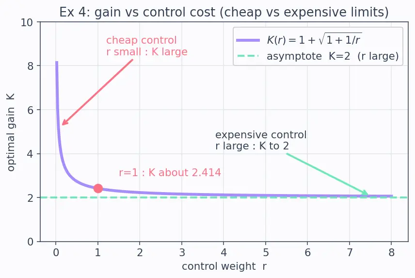
2. Gain as a function of $r$. $K(r)=\frac{b}{r}p=\frac{r+\sqrt{r^2+r}}{r}=1+\sqrt{1+\frac{1}{r}}$. Why write it this way? Dividing by $r$ (and pulling $r$ inside the root: $\sqrt{r^2+r}/r=\sqrt{1+1/r}$) isolates the $\frac{1}{r}$ term whose limit we can read off directly.

3. Cheap control, $r\to 0^{+}$. $\frac{1}{r}\to \infty$, so $K\to \infty$. Why? Control is almost free, so the optimizer spends unlimited effort → infinite gain → the pole $a-bK\to -\infty$ (instant correction). This is the D-cell limit.

4. Expensive control, $r\to \infty$. $\frac{1}{r}\to 0$, so $K\to 1+\sqrt{1}=2$; pole $a-bK\to 1-2=-1$. Why not $K\to 0$? Because $a=1$ is unstable — you can never fully stop spending, or the state runs away. The controller settles at the cheapest gain that still stabilizes, mirroring the plant's own rate. This mirror-image pole ($-|a|$) is a famous LQR fact (cheap-vs-expensive limit).

5. Figure.

   

   The horizontal axis is the control weight $r$ (from $0$ to $8$); the vertical axis is the optimal gain $K$. The lavender curve $K(r)=1+\sqrt{1+1/r}$ dives from $+\infty$ on the left down to the mint dashed asymptote at $K=2$ on the right; the coral dot marks the value $K(1)\approx 2.414$.

Verify: at $r=1$, $K=1+\sqrt{2}\approx 2.414$ — matches the parent note's worked number exactly. ✔ The two asymptotes ($K\to \infty$ and $K\to 2$) bracket it correctly.

---

Example 5 — Cell H: only the ratio $Q/R$ matters (aggressiveness)

Forecast: scaling both penalties by the same factor — does the controller get more aggressive, less, or unchanged?

1. General gain in terms of the ratio. With $a=b=1$ the positive root (from the box) is $p=r+\sqrt{r^2+qr}$, so $K=\frac{p}{r}=1+\sqrt{1+\frac{q}{r}}.$ Why this step? Factor $r$ out of the square root: $\sqrt{r^2+qr}=r\sqrt{1+q/r}$. After dividing by $r$, only the ratio $q/r$ survives — no standalone $q$ or $r$ remains.

2. Case $(1,1)$: $q/r=1$, so $K=1+\sqrt{2}\approx 2.414$.

3. Case $(100,100)$: $q/r=1$ again, so $K=1+\sqrt{2}\approx 2.414$. Identical.

Verify: the two gains are numerically equal because $K$ depends only on $q/r$. This confirms the parent-note mistake #1: only the ratio sets aggressiveness, scaling both is a no-op. ✔

---

Example 6 — Cell F: double integrator, LQR = PD controller

Forecast: LQR here becomes a PD controller. What damping ratio should we expect?

1. Expand the CARE entry by entry (done here, not assumed). With $A^{\top }P+PA-PB{R}^{-1}{B}^{\top }P+Q=0$ and $B^{\top }P=[p_2,p_3]$, so $PB{R}^{-1}{B}^{\top }P=\frac{1}{\rho }\left[\begin{array}{cc}{p}_2^2& p_2{p}_3\\ p_2{p}_3& p_3^2\end{array}\right]$, the three scalar equations are:

   • $(1,1)$: $1-p_2^2/\rho =0$,
   • $(1,2)$: $p_1-p_2{p}_3/\rho =0$,
   • $(2,2)$: $2p_2-p_3^2/\rho =0$. Why this step? A symmetric $2\times 2$ matrix equation gives exactly three independent scalar equations — one per distinct entry — which we solve in order.

2. Solve them. From $(1,1)$: $p_2=\sqrt{\rho }$. From $(2,2)$: $p_3=\sqrt{2\rho p_2}=\sqrt{2}{\rho }^{3/4}$. From $(1,2)$: $p_1=p_2{p}_3/\rho$. With $\rho =1$: $p_2=1,p_3=\sqrt{2},p_1=\sqrt{2}$.

3. Gain. $K=\frac{1}{\rho }[p_2,p_3]=[1,\sqrt{2}]$. So $k_p=1$ (position/spring), $k_d=\sqrt{2}$ (velocity/damper). Why is this PD? $u=-k_p{x}_1-k_d{x}_2=-(\text{spring})x_1-(\text{damper})x_2$ — the textbook PD form (see PID Controllers, Pole Placement).

4. Closed-loop matrix. $A-BK=\left[\begin{array}{cc}0& 1\\ -1& -\sqrt{2}\end{array}\right]$. Characteristic poly: $s^2+\sqrt{2}s+1=0$. Why? $\det (sI-(A-BK))=s(s+\sqrt{2})+1$.

5. Poles. $s=\frac{-\sqrt{2}\pm \sqrt{2-4}}{2}=-\frac{1}{\sqrt{2}}\pm j\frac{1}{\sqrt{2}}$.

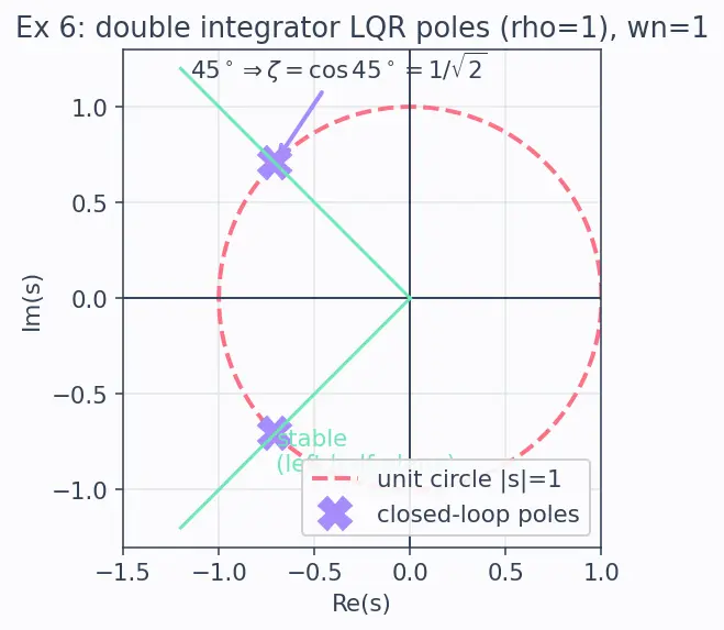
6. Figure.

   

   The axes are the complex $s$-plane: horizontal = real part $\text{Re}(s)$, vertical = imaginary part $\text{Im}(s)$. The two lavender crosses are the closed-loop poles at $-1/\sqrt{2}\pm j/\sqrt{2}$; they sit on the coral unit circle ($|s|=1$) at $45^{\circ }$ into the left half-plane — damping ratio $\zeta =\cos 45^{\circ }=1/\sqrt{2}$.

Verify: ${\omega }_n=|s|=\sqrt{(1/\sqrt{2}{)}^2+(1/\sqrt{2}{)}^2}=1$, and $\zeta =1/\sqrt{2}\approx 0.707$ — the "critically nice" GNC damping. ✔

---

Example 7 — Cell F (twist): expensive control on the double integrator

Forecast: more expensive control should mean smaller gains and a slower (lower-frequency) response. By what factor?

1. Plug $\rho =16$ into the general entries from Example 6. $p_2=\sqrt{\rho }=4$, $p_3=\sqrt{2}{\rho }^{3/4}=\sqrt{2}\cdot 8=8\sqrt{2}$. Why? ${\rho }^{3/4}=16^{3/4}=(2^4{)}^{3/4}=2^3=8$.

2. Gain. $K=\frac{1}{\rho }[p_2,p_3]=\frac{1}{16}[4,8\sqrt{2}]=[0.25,0.5\sqrt{2}]=[0.25,0.7071]$.

3. Natural frequency. For LQR on this plant, ${\omega }_n=\sqrt{k_p}=\sqrt{1/\sqrt{\rho }}={\rho }^{-1/4}=16^{-1/4}=0.5$. Why? Closed-loop poly is $s^2+k_{d}s+k_p$, so ${\omega }_n=\sqrt{k_p}=\sqrt{0.25}=0.5$.

Verify: compared to Example 6 (${\omega }_n=1$), $\rho$ grew by $16\times$ and ${\omega }_n$ dropped by $16^{1/4}=2\times$ (from $1$ to $0.5$). Slower and gentler, exactly as "expensive control" predicts. Damping check: $\zeta =k_d/(2{\omega }_n)=0.7071/(2\cdot 0.5)=0.7071=1/\sqrt{2}$ — same damping ratio (a scale-invariance of this problem). ✔

---

Example 8 — Cell G: degenerate $Q$ that is still OK

Forecast: $Q$ has a zero eigenvalue, so we penalize nothing about velocity directly. Does the solution still stabilize both states?

1. State the requirement. A stabilizing $P⪰0$ exists iff $(A,B)$ controllable and $(A,\sqrt{Q})$ observable (Controllability and Observability). Why this step? A degenerate $Q$ is fine as long as the penalized quantity "sees" every unstable mode through the dynamics.

2. Pick $\sqrt{Q}$. As defined above, $\sqrt{Q}=C=\left[\begin{array}{cc}1& 0\\ 0& 0\end{array}\right]$, i.e. output $=x_1$ (position).

3. Observability of $(A,C)$. $\mathcal{O}=\left[\begin{array}{c}C\\ CA\end{array}\right]=\left[\begin{array}{cc}1& 0\\ 0& 1\end{array}\right]$, rank 2 = full. Why does this rescue us? Even though we don't penalize velocity directly, velocity is observable from position through $CA$ (position's rate reveals velocity). So the cost still "feels" a runaway velocity.

4. Consequence. The Example-6 solution $K=[1,\sqrt{2}]$ is valid and stabilizing despite the degenerate $Q$.

Verify: the observability matrix is the $2\times 2$ identity, determinant $=1\ne 0$ ⇒ full rank ⇒ LQR well-posed. ✔ (Contrast this with Cell I next, where the plant itself fails a condition.)

---

Example 9 — Cell I: when the recipe refuses to work

Forecast: the control $u$ enters only the first row. The unstable mode is $x_2$. Can any gain touch it?

1. Build the controllability matrix. $\mathcal{C}=[B,AB]$. $AB=\left[\begin{array}{cc}0& 0\\ 0& 1\end{array}\right]\left[\begin{array}{c}1\\ 0\end{array}\right]=\left[\begin{array}{c}0\\ 0\end{array}\right]$. So $\mathcal{C}=\left[\begin{array}{cc}1& 0\\ 0& 0\end{array}\right]$. Why this step? $(A,B)$ controllable ⇔ $\mathcal{C}$ has full rank $n=2$ (Controllability and Observability).

2. Rank. $\det \mathcal{C}=0$, rank $=1<2$. Uncontrollable.

3. Diagnose which mode. The uncontrollable mode is $x_2$, whose eigenvalue is $+1$ (unstable). An unstable and uncontrollable mode cannot be moved by any $u=-Kx$. Why does this kill LQR? No feedback gain can push a pole the control cannot reach. The Riccati equation will not yield a stabilizing $P⪰0$.

4. Conclusion. LQR has no stabilizing solution here; you must redesign the actuator ($B$) so it couples into $x_2$.

Verify: $\det \mathcal{C}=1\cdot 0-0\cdot 0=0$ ⇒ rank-deficient ⇒ uncontrollable. The recipe correctly fails. ✔ This is the boundary case every LQR user must recognize.

---

Example 10 — Cell J: satellite design word problem

Forecast: we found ${\omega }_n={\rho }^{-1/4}$. To slow down to $0.5$, do we make $\rho$ big or small?

1. Invert the frequency relation. From Example 7, ${\omega }_n={\rho }^{-1/4}$, so $\rho ={\omega }_n^{-4}=(0.5{)}^{-4}=16$. Why this step? We derived ${\omega }_n={\rho }^{-1/4}$; solving for $\rho$ gives the required control weight. A large $\rho$ (expensive control) ⇒ slow response — matching the forecast.

2. Compute the gain (reuse Example 7). $K=[0.25,0.7071]$.

3. Engineering reading. $k_p=0.25$ (torque per radian) = the restoring "spring"; $k_d=0.707$ (torque per rad/s) = the damping. Damping ratio $\zeta =1/\sqrt{2}\approx 0.707$ → about $5\%$ overshoot, a smooth slew. Why is this good for a satellite? Low ${\omega }_n$ ⇒ gentle wheel torques ⇒ less power and less structural stress, at the cost of a slower settle. See LQG Control for when the state must be estimated first.

Verify: $\rho =16\Rightarrow {\omega }_n=16^{-1/4}=0.5$ ✔; $K=[0.25,0.7071]$ ✔ (identical to Example 7, as it must be — same $\rho$).

---

Recall Coverage checklist (did we hit every cell?)

A ✔ (Ex 1) · B ✔ (Ex 2) · C ✔ (Ex 3) · D & E ✔ (Ex 4) · H ✔ (Ex 5) · F ✔ (Ex 6, 7) · G ✔ (Ex 8) · I ✔ (Ex 9) · J ✔ (Ex 10). Stable/unstable/marginal scalars, cheap/expensive limits, ratio-invariance, matrix PD case, degenerate-but-OK $Q$, and the uncontrollable failure — all shown.

Active Recall