Worked examples — Uniform continuity — difference from pointwise

This page is a workout. The parent note built the ideas; here we drill every kind of case the topic can throw at you until none is unfamiliar. If a word or symbol looks new, we re-earn it on the spot.

Two symbols we use constantly, spelled out in words:

• $\epsilon$ (epsilon) — the output tolerance: how close the two heights are allowed to differ. "Up–down" distance.
• $\delta$ (delta) — the input closeness we are allowed to demand. "Sideways" distance.
• $|x-y|$ — the sideways gap; $|f(x)-f(y)|$ — the up–down gap. The vertical bars mean "distance, always positive".

---

The scenario matrix

Every uniform-continuity question falls into one of these cells. The examples below hit each one, and the label after each example name tells you which cell.

Cell	What makes it that cell	Example
A. Bounded compact domain	closed & bounded $[a,b]$ — Heine–Cantor guarantees UC	Ex 1
B. Unbounded domain, amplifier grows	$	x+y
C. Bounded but NOT closed, blow-up at open end	$(0,1)$, $1/x$ near $0$ → fails	Ex 3
D. Non-Lipschitz yet still UC	slope $\to \infty$ but tamed by a root bound	Ex 4
E. Lipschitz constant hunt (uses MVT)	bounded derivative → explicit $\delta =\epsilon /L$	Ex 5
F. Oscillation degenerate case	$\sin (1/x)$ on $(0,1)$ — bounded output, still fails	Ex 6
G. Limiting / boundary-repair	extend to an endpoint to restore UC	Ex 7
H. Real-world word problem	temperature-sensor closeness rule	Ex 8
I. Exam twist: sum/product of UC	is $x\sin x$ UC on $\mathbb{R}$?	Ex 9

We will also touch the degenerate zero cases (constant function, single-point domain) inside Ex 1.

---

Ex 1 — Cell A: compact domain, and the degenerate zeros

Forecast: guess — on a finite closed stretch, does one $\delta$ survive? Write your bet before reading.

1. WHAT: write the output gap using the amplifier factorisation. $|x^2-y^2|=|x+y||x-y|.$ Why this step? Factoring exposes the multiplier $|x+y|$ that turns an input gap into an output gap — the whole behaviour lives in that factor.

2. WHAT: bound the amplifier on this domain. Since $0\le x,y\le 5$, $|x+y|\le 5+5=10.$ Why this step? Because the domain is bounded, the dangerous factor is capped by a fixed number — no dependence on where we are. That is the seed of uniformity.

3. WHAT: choose $\delta$. Take $\delta =\frac{\epsilon }{10}$. Then $|x-y|<\delta ⟹|x^2-y^2|\le 10|x-y|<10\cdot \frac{\epsilon }{10}=\epsilon .$ Why this step? $\delta$ contains only $\epsilon$ and the number $10$ — no $x$. That "no $x$" is literally the definition of uniform continuity.

4. Degenerate zeros.

   • Constant $f(x)=c$: output gap is always $0$, so any $\delta$ works — vacuously uniformly continuous.
   • One-point domain $A=\{p\}$: the only pair is $x=y=p$, gap $0$ — again vacuously UC. Why this step? Extreme inputs must never surprise us; here they are the easiest cases, not exceptions.

Verify: pick $\epsilon =0.1\Rightarrow \delta =0.01$. Take the worst nearby pair $x=5,y=4.99$: $|x-y|=0.01$, and $|x^2-y^2|=|25-24.9001|=0.0999<0.1$. ✓

---

Ex 2 — Cell B: unbounded domain, amplifier explodes

Forecast: which grows faster as we march right — the input gap we're allowed, or the output gap it produces?

1. WHAT: fix the target $\epsilon =1$. Suppose a rescuer hands us some $\delta >0$. Why this step? To negate "there exists a $\delta$", we defeat an arbitrary $\delta$.

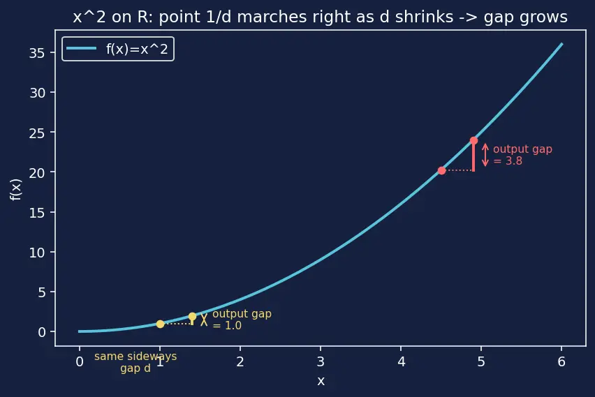
2. WHAT: engineer the pair $x=\frac{1}{\delta },y=\frac{1}{\delta }+\frac{\delta }{2}.$ Their gap is $|x-y|=\frac{\delta }{2}<\delta$ — legally close. See

   

   (figure: the $x^2$ parabola with a yellow pair at $x=1/\delta$ for a larger $\delta$ and a red pair at $x=1/\delta$ for a smaller $\delta$ — both a fixed sideways gap apart; the red vertical output gap is visibly far taller — showing that as $\delta$ shrinks the engineered point $1/\delta$ marches right into steeper territory). Why this step? We place the pair far out where the slope is huge, keeping them sideways-close.

3. WHAT: compute the output gap. $|x^2-y^2|=|x+y||x-y|=(\frac{2}{\delta }+\frac{\delta }{2})\cdot \frac{\delta }{2}=1+\frac{{\delta }^2}{4}>1=\epsilon .$ Why this step? The output gap exceeds $\epsilon$ no matter how small $\delta$ was — the negation is complete.

Verify: $\delta =0.1\Rightarrow x=10,y=10.05$: $|x-y|=0.05<0.1$ ✓, and $|x^2-y^2|=|100-101.0025|=1.0025>1$ ✓.

---

Ex 3 — Cell C: bounded but not closed, blow-up at an open end

Forecast: "bounded" felt safe in Ex 1 — why might it fail here?

1. WHAT: note $(0,1)$ is not closed: the point $0$ is missing, and $f\to \infty$ as $x\to 0^{+}$. Why this step? Heine–Cantor Theorem needs closed AND bounded (Compactness). Missing $0$ breaks closedness, so no guarantee — we test directly.

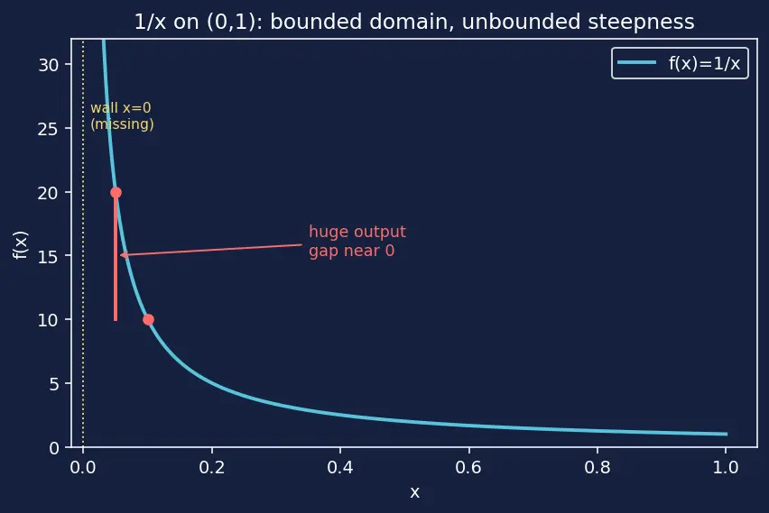
2. WHAT: fix $\epsilon =1$; take any $\delta >0$; pick points hugging $0$: $x=\delta ,y=\frac{\delta }{2}(\text{both in }(0,1)\text{ for small }\delta ).$ Gap $|x-y|=\delta /2<\delta$. See

   

   (figure: the $1/x$ curve rocketing upward as it approaches the yellow dotted wall at $x=0$; a red pair of points near the wall shows a tiny sideways step producing a huge vertical leap). Why this step? The steepness lives near $0$, so we crowd the pair against that wall.

3. WHAT: measure the output gap. $|\frac{1}{x}-\frac{1}{y}|=|\frac{1}{\delta }-\frac{2}{\delta }|=\frac{1}{\delta }.$ For $\delta <1$ this is $>1=\epsilon$. Why this step? Output gap $1/\delta \to \infty$ as $\delta \to 0$ — beats any tolerance, so no single $\delta$ works.

Verify: $\delta =0.1\Rightarrow x=0.1,y=0.05$: $|x-y|=0.05<0.1$ ✓, $|1/x-1/y|=|10-20|=10>1$ ✓.

---

Ex 4 — Cell D: non-Lipschitz yet uniformly continuous

Forecast: the slope $\frac{1}{2\sqrt{x}}\to \infty$ near $0$ — same warning sign as $1/x$. Why does $\sqrt{x}$ survive where $1/x$ died?

1. WHAT: Lipschitz would need a fixed $L$ with $|\sqrt{x}-\sqrt{y}|\le L|x-y|$. Near $0$ the derivative $f^{\prime }(x)=\frac{1}{2\sqrt{x}}\to \infty$, so no finite $L$ exists. Why this step? We first admit the easy test fails — Lipschitz is sufficient, not necessary.

2. WHAT: prove the square-root inequality from scratch. Assume WLOG $x\ge y\ge 0$, so $\sqrt{x}\ge \sqrt{y}\ge 0$. Compare $(\sqrt{x}-\sqrt{y}{)}^2$ against $x-y=(\sqrt{x}-\sqrt{y})(\sqrt{x}+\sqrt{y})$: $(\sqrt{x}-\sqrt{y}{)}^2=(\sqrt{x}-\sqrt{y})(\sqrt{x}-\sqrt{y})\le (\sqrt{x}-\sqrt{y})(\sqrt{x}+\sqrt{y})=x-y,$ because $\sqrt{x}-\sqrt{y}\le \sqrt{x}+\sqrt{y}$ (we only added the non-negative $2\sqrt{y}$ to the second factor while the first factor $\sqrt{x}-\sqrt{y}\ge 0$). Taking square roots of $(\sqrt{x}-\sqrt{y}{)}^2\le |x-y|$ gives $|\sqrt{x}-\sqrt{y}|\le \sqrt{|x-y|}.$ Why this step? This is the engine of the whole example, so we derive it rather than quote it: replacing the smaller factor $(\sqrt{x}-\sqrt{y})$ by the larger $(\sqrt{x}+\sqrt{y})$ can only increase the product, and that larger product is exactly $x-y$.

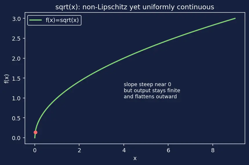
3. WHAT: read off the growth. The output gap grows only like $\sqrt{\text{input gap}}$ — a gentler growth. Unlike $1/x$, the function stays bounded and finite everywhere, including at $0$; its graph flattens (not steepens) as $x$ grows. Compare the mild slope in

   

   (figure: the green $\sqrt{x}$ curve rising steeply from the origin then flattening; a red dot near $0$ marks where the slope is largest, yet the output stays finite).

4. WHAT: choose $\delta ={\epsilon }^2$. Then $|x-y|<{\epsilon }^2⟹|\sqrt{x}-\sqrt{y}|\le \sqrt{|x-y|}<\sqrt{{\epsilon }^2}=\epsilon .$ Why this step? $\delta$ depends on $\epsilon$ alone — uniformity achieved without Lipschitz.

Verify: $\epsilon =0.1\Rightarrow \delta =0.01$. Worst near-$0$ pair $x=0.01,y=0$: $|x-y|=0.01=\delta$ (boundary), $|\sqrt{x}-\sqrt{y}|=0.1$, which is $\le \epsilon$. ✓

---

Ex 5 — Cell E: hunt the Lipschitz constant via the Mean Value Theorem

Forecast: $\sin$ wiggles forever — does "forever" break uniformity like $x^2$ did?

1. WHAT: compute the derivative and bound it. $f^{\prime }(x)=\cos x$, and $|\cos x|\le 1$ for all $x$. Why this step? A bounded slope is the cleanest route to Lipschitz. Here $L=1$ — a single number for the whole line.

2. WHAT: invoke the Mean Value Theorem. For any $x,y$ there is a $c$ between them with $\sin x-\sin y=\cos c(x-y)\Rightarrow |\sin x-\sin y|=|\cos c||x-y|\le 1\cdot |x-y|.$ Why this step? MVT converts "bounded derivative" into "bounded output-to-input ratio", i.e. Lipschitz with $L=1$.

3. WHAT: choose $\delta =\epsilon$ (since $\delta =\epsilon /L=\epsilon /1$). $|x-y|<\epsilon ⟹|\sin x-\sin y|\le |x-y|<\epsilon .$ Why this step? No $x$ in $\delta$ — uniform, even though the graph never stops oscillating. The wiggle is bounded in height and steepness, unlike $x^2$'s ever-growing steepness.

Verify: $\epsilon =0.05\Rightarrow \delta =0.05$. Take $x=0,y=0.05$: $|\sin x-\sin y|=|\sin 0.05|=0.049979<0.05$ ✓.

---

Ex 6 — Cell F: bounded oscillation that STILL fails

Forecast: the output never leaves $[-1,1]$ — so how can output gaps blow past $\epsilon$?

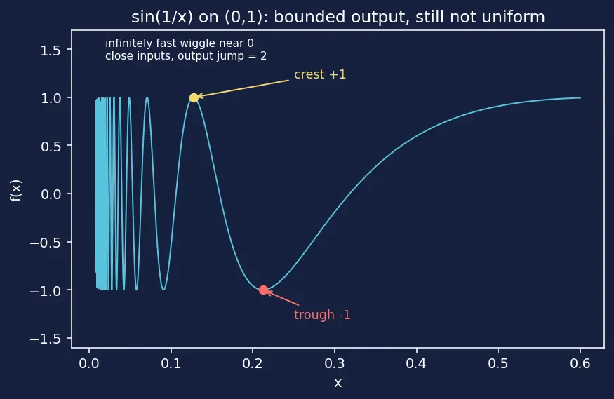
1. WHAT: fix $\epsilon =1$; take any $\delta >0$. Choose two peaks/valleys of the wiggle near $0$, indexed by a positive integer $n$: $x_n=\frac{1}{2\pi n+\frac{\pi }{2}},y_n=\frac{1}{2\pi n-\frac{\pi }{2}}.$ Then $f(x_n)=\sin (2\pi n+\frac{\pi }{2})=1$ and $f(y_n)=\sin (2\pi n-\frac{\pi }{2})=-1$. Why this step? Near $0$ the graph oscillates infinitely fast, so a $+1$ crest and a $-1$ trough sit arbitrarily close together — see

   

   (figure: the blue $\sin (1/x)$ curve wiggling faster and faster toward $0$; a yellow dot marks a $+1$ crest and a red dot a nearby $-1$ trough, so two close inputs give an output jump of $2$).

2. WHAT: check domain membership. For every integer $n\ge 1$ the denominators satisfy $2\pi n-\frac{\pi }{2}>2\pi \cdot 1-\frac{\pi }{2}=\frac{3\pi }{2}>1$, so both $x_n,y_n\in (0,\frac{2}{3\pi })\subset (0,1)$. Every $n\ge 1$ is legal; no smallness assumption is needed. Why this step? We must confirm the engineered points actually live in the domain before using them, and here even $n=1$ already lands safely inside $(0,1)$.

3. WHAT: estimate the sideways gap so we can beat any $\delta$. Subtracting the two fractions over a common denominator, $|x_n-y_n|=\left|\frac{1}{2\pi n+\frac{\pi }{2}}-\frac{1}{2\pi n-\frac{\pi }{2}}\right|=\frac{\pi }{\left(2\pi n+\frac{\pi }{2}\right)\left(2\pi n-\frac{\pi }{2}\right)}=\frac{\pi }{(2\pi n{)}^2-{\left(\frac{\pi }{2}\right)}^2}\underset{n\to \infty }{\to }0.$ So given any $\delta >0$, pick $n$ large enough that this quantity is $<\delta$; both points still lie in $(0,1)$ by step 2. Why this step? The explicit formula $\frac{\pi }{(2\pi n{)}^2-(\pi /2{)}^2}$ proves the crests bunch up at $0$ — we don't just assert it.

4. WHAT: yet the output gap is $|f(x_n)-f(y_n)|=|1-(-1)|=2>1=\epsilon .$ Why this step? Bounded output does not save you — what matters is that close inputs can still give a fixed jump of $2$. Frequency, not amplitude, kills uniformity.

Verify (n=1): $x_1=1/(2\pi +\pi /2)\approx 0.1273$, $y_1=1/(2\pi -\pi /2)\approx 0.1819$; $|x_1-y_1|\approx 0.0546<0.1$, output gap $=2>1$ ✓.

---

Ex 7 — Cell G: limiting/boundary repair restores UC

Forecast: can plugging a single missing point turn a "maybe" into a guaranteed UC — and can we still write a concrete closeness rule?

1. WHAT: compute the limit at the open end. ${\lim }_{x\to 0^{+}}\frac{\sin x}{x}=1.$ Why this step? The only thing stopping compactness was the missing endpoint $0$. If the function has a finite limit there, we can fill the hole continuously.

2. WHAT: set $g(0)=1$. Now $g$ is continuous on the closed bounded interval $[0,1]$. Why this step? $[0,1]$ is compact; unlike Ex 3's open $(0,1)$, nothing runs off to infinity.

3. WHAT (qualitative): apply Heine–Cantor Theorem: continuous on a compact set $\Rightarrow$ uniformly continuous. Why this step? We converted a boundary defect into a compact domain, and the theorem does the rest.

4. WHAT (quantitative $\delta$): we build $\delta$ by hand, and we prove the slope bound rather than assert it. Write $g^{\prime }(x)=\frac{x\cos x-\sin x}{x^2}$ for $x>0$ (and $g^{\prime }(0)=0$ by symmetry, since $g$ is even). Use the two standard inequalities valid for $x\in (0,1]$: $\sin x\ge x-\frac{x^3}{6},\cos x\le 1.$ Then the numerator obeys $x\cos x-\sin x\le x\cdot 1-(x-\frac{x^3}{6})=\frac{x^3}{6},$ and (using $\sin x\le x$, $\cos x\ge 1-\frac{x^2}{2}$) it also obeys $x\cos x-\sin x\ge x(1-\frac{x^2}{2})-x=-\frac{x^3}{2}$. Hence $|g^{\prime }(x)|=\frac{|x\cos x-\sin x|}{x^2}\le \frac{\max (\frac{x^3}{6},\frac{x^3}{2})}{x^2}=\frac{x}{2}\le \frac{1}{2}\text{for }x\in (0,1].$ So $|g^{\prime }|\le \frac{1}{2}$ on all of $[0,1]$. By the Mean Value Theorem this gives Lipschitz constant $L=\frac{1}{2}$, so $\delta =\frac{\epsilon }{L}=2\epsilon ,|x-y|<2\epsilon \Rightarrow |g(x)-g(y)|\le \frac{1}{2}|x-y|<\epsilon .$ Why this step? Heine–Cantor guarantees a $\delta$; the Taylor-type bounds $\sin x\ge x-\frac{x^3}{6}$ and $\cos x\ge 1-\frac{x^2}{2}$ turn "one checks" into a genuine everywhere-valid inequality $|g^{\prime }|\le \frac{x}{2}\le \frac{1}{2}$, handing us an explicit $\delta$.

Verify: the limit numerically: $\sin (0.001)/0.001=0.99999983\approx 1$ ✓; and the bound: the actual maximum of $|g^{\prime }|$ on $[0,1]$ is at $x=1$, $|g^{\prime }(1)|\approx 0.30\le \frac{1}{2}$, consistent with our proven bound $|g^{\prime }(x)|\le x/2$ ✓, so $L=\frac{1}{2}$ is a safe (loose) Lipschitz constant.

---

Ex 8 — Cell H: real-world word problem

Forecast: does one closeness rule cover the whole run, or must it change over time?

1. WHAT: find the steepest rate of change (bound the derivative). $T^{\prime }(t)=3-\frac{1}{5}t,|T^{\prime }(t)|\le \max (|T^{\prime }(0)|,|T^{\prime }(10)|)=\max (3,1)=3\frac{{}^{\circ }\text{C}}{\text{min}}.$ Why this step? Bounded slope $L=3$ on the compact interval $[0,10]$ gives Lipschitz via Mean Value Theorem — the physical version of "one rule everywhere".

2. WHAT: Lipschitz bound: $|T(s)-T(t)|\le 3|s-t|$. Why this step? Turns "how fast can temperature move" into "how far apart two readings can be".

3. WHAT: solve $3\delta =\epsilon$: $\delta =\frac{\epsilon }{L}=\frac{0.5}{3}\approx 0.1667$ minutes ($\approx 10$ seconds). Why this step? $\delta$ depends only on the tolerance and the slope bound — not on which minute we sample. Uniformity = one compliance rule for the whole shift.

Verify: worst case near $t=0$ (steepest): $T(0)=20$, $T(0.1667)=20+0.5-0.00278=20.497$; gap $=0.497<0.5$ ✓. Units: $\frac{{}^{\circ }\text{C}}{\text{min}}\times \text{min}={}^{\circ }\text{C}$ ✓.

---

Ex 9 — Cell I: exam twist on products

Forecast: it is tempting to think "product of two well-behaved functions must be well-behaved." Bet yes or no before reading — the exam trap is that the answer is no.

1. WHAT: test the derivative for a growing slope. $f^{\prime }(x)=\sin x+x\cos x,|f^{\prime }(x)|\ge |x\cos x|-|\sin x|.$ At $x=2\pi n$: $\cos (2\pi n)=1,\sin (2\pi n)=0$, so $f^{\prime }(2\pi n)=2\pi n\to \infty$. Why this step? An unbounded slope is the classic warning flag (recall $x^2$). The factor $x$ amplifies the oscillation's steepness without limit — so we suspect failure and go hunting for bad pairs.

2. WHAT: engineer sideways-close, output-far pairs. Near $x_n=2\pi n$ (where $\sin =0$, so $f(x_n)=0$) take a nearby point $y_n=2\pi n+h$ with a fixed small $h$: $f(y_n)=(2\pi n+h)\sin (2\pi n+h)=(2\pi n+h)\sin h.$ The sideways gap is $|x_n-y_n|=h$; choose $h<\delta$ so it is legally close. Then $|f(y_n)-f(x_n)|=(2\pi n+h)|\sin h|\ge 2\pi n|\sin h|\underset{n\to \infty }{\to }\infty .$ Why this step? With $h$ fixed the sideways gap never changes, but $2\pi n|\sin h|$ grows without bound as $n\to \infty$ — this is the exact negation pattern from Ex 2.

3. WHAT: conclude. For any candidate $\delta >0$ pick $h=\min (\delta /2,1)$ (so $h<\delta$ and $\sin h\ne 0$), then pick $n$ large enough that $2\pi n|\sin h|>\epsilon$. Two points closer than $\delta$ with output gap above $\epsilon$ exist ⇒ $x\sin x$ is not uniformly continuous on $\mathbb{R}$. There is no rescuing $\delta (\epsilon )$. Why this step? Moral: uniform continuity is not closed under multiplication on unbounded domains — a genuine exam trap. (On any bounded $[a,b]$ it is fine, by Heine–Cantor.)

Verify: take $h=0.1$, $n=100$ so $x=200\pi \approx 628.3185$, $y=x+0.1$: $|x-y|=0.1$, and $|f(x)-f(y)|=|0-(628.4185)\sin (628.4185)|\approx 62.75\gg \epsilon$. Doubling $n$ roughly doubles this gap ⇒ unbounded ✓.

---

Recall Scenario checklist to run on any function

Compact domain? → UC free (Heine–Cantor). Bounded derivative? → Lipschitz, $\delta =\epsilon /L$. Slope $\to \infty$ or domain unbounded / open at a blow-up? → hunt bad pairs (crowd them where it's steep). Bounded output but infinite oscillation? → still can fail (Ex 6). Missing endpoint with a finite limit? → fill it and gain compactness (Ex 7).

Connections

• Continuity (pointwise) — the weaker property every example starts from.
• Heine–Cantor Theorem — powers Ex 1 and Ex 7.
• Compactness / Lebesgue number lemma — why closed+bounded rescues.
• Lipschitz continuity — Ex 5, Ex 8 (and Ex 4 shows it's not necessary).
• Mean Value Theorem — bounded slope → Lipschitz, used in Ex 5, Ex 7 & Ex 8.
• Cauchy sequences — UC preserves Cauchyness, the deeper reason $1/x$ fails on $(0,1)$.