Worked examples — Uniform continuity — difference from pointwise

4.10.23 · D3 · Maths › Advanced Topics (Elite Level) › Uniform continuity — difference from pointwise

Yeh page ek workout hai. Parent note ne ideas build kiye the; yahan hum har tarah ke case drill karte hain jo yeh topic throw kar sakta hai, jab tak koi bhi unfamiliar na lage. Agar koi word ya symbol naya lagta hai, hum usse wahi pe re-earn karte hain.

Do symbols jo hum constantly use karte hain, words mein:

• $\epsilon$ (epsilon) — output tolerance: do heights kitni close allowed hain differ karne ke liye. "Upar–neeche" distance.
• $\delta$ (delta) — input closeness jo hum demand kar sakte hain. "Sideways" distance.
• $|x-y|$ — sideways gap; $|f(x)-f(y)|$ — upar–neeche gap. Vertical bars ka matlab hai "distance, hamesha positive".

---

Scenario matrix

Har uniform-continuity question in cells mein se ek mein aata hai. Neeche ke examples har ek ko hit karte hain, aur har example name ke baad label batata hai ki kaunsa cell hai.

Cell	Kya cheez isse woh cell banati hai	Example
A. Bounded compact domain	closed & bounded $[a,b]$ — Heine–Cantor UC guarantee karta hai	Ex 1
B. Unbounded domain, amplifier grows	$	x+y
C. Bounded but NOT closed, blow-up at open end	$(0,1)$, $1/x$ near $0$ → fails	Ex 3
D. Non-Lipschitz yet still UC	slope $\to \infty$ but ek root bound se tamed	Ex 4
E. Lipschitz constant hunt (uses MVT)	bounded derivative → explicit $\delta =\epsilon /L$	Ex 5
F. Oscillation degenerate case	$\sin (1/x)$ on $(0,1)$ — bounded output, phir bhi fails	Ex 6
G. Limiting / boundary-repair	endpoint pe extend karke UC restore karo	Ex 7
H. Real-world word problem	temperature-sensor closeness rule	Ex 8
I. Exam twist: sum/product of UC	kya $x\sin x$ UC hai $\mathbb{R}$ pe?	Ex 9

Hum degenerate zero cases (constant function, single-point domain) bhi Ex 1 ke andar touch karenge.

---

Ex 1 — Cell A: compact domain, aur degenerate zeros

Forecast: andaaza lagao — kya ek finite closed stretch pe ek $\delta$ survive karta hai? Padhne se pehle apna bet likhо.

1. WHAT: output gap ko amplifier factorisation se likho. $|x^2-y^2|=|x+y||x-y|.$ Yeh step kyun? Factor karne se multiplier $|x+y|$ expose hota hai jo ek input gap ko output gap mein turn karta hai — poora behaviour us factor mein rehta hai.

2. WHAT: is domain pe amplifier ko bound karo. Kyunki $0\le x,y\le 5$, $|x+y|\le 5+5=10.$ Yeh step kyun? Kyunki domain bounded hai, woh dangerous factor ek fixed number se capped hai — koi dependence nahi hai ki hum kahan hain. Yahi uniformity ka seed hai.

3. WHAT: $\delta$ choose karo. $\delta =\frac{\epsilon }{10}$ lo. Tab $|x-y|<\delta ⟹|x^2-y^2|\le 10|x-y|<10\cdot \frac{\epsilon }{10}=\epsilon .$ Yeh step kyun? $\delta$ mein sirf $\epsilon$ aur number $10$ hai — koi $x$ nahi. Yoh "no $x$" literally uniform continuity ki definition hai.

4. Degenerate zeros.

   • Constant $f(x)=c$: output gap hamesha $0$ hota hai, toh koi bhi $\delta$ kaam karta hai — vacuously uniformly continuous.
   • One-point domain $A=\{p\}$: sirf ek pair hai $x=y=p$, gap $0$ — again vacuously UC. Yeh step kyun? Extreme inputs hume kabhi surprise nahi karne chahiye; yahan woh sabse aasaan cases hain, exceptions nahi.

Verify: $\epsilon =0.1\Rightarrow \delta =0.01$ lo. Worst nearby pair $x=5,y=4.99$ lo: $|x-y|=0.01$, aur $|x^2-y^2|=|25-24.9001|=0.0999<0.1$. ✓

---

Ex 2 — Cell B: unbounded domain, amplifier explodes

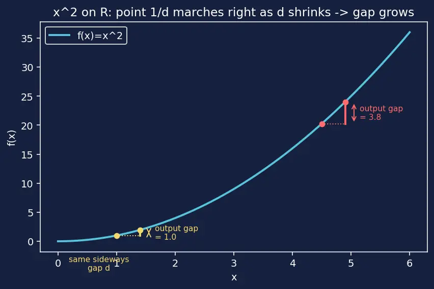
Forecast: jaise-jaise hum right march karte hain — kaunsa zyada fast grow karta hai — woh input gap jo hum allowed hain, ya woh output gap jo woh produce karta hai?

1. WHAT: target $\epsilon =1$ fix karo. Maano ek rescuer humein koi $\delta >0$ deta hai. Yeh step kyun? "There exists a $\delta$" ko negate karne ke liye, hum ek arbitrary $\delta$ ko defeat karte hain.

2. WHAT: pair engineer karo $x=\frac{1}{\delta },y=\frac{1}{\delta }+\frac{\delta }{2}.$ Unka gap hai $|x-y|=\frac{\delta }{2}<\delta$ — legally close. Dekho

   

   (figure: $x^2$ parabola jisme ek bade $\delta$ ke liye $x=1/\delta$ pe yellow pair aur ek chhote $\delta$ ke liye $x=1/\delta$ pe red pair hai — dono ek fixed sideways gap apart; red vertical output gap visibly kaafi zyada tall hai — dikhata hai ki jaise $\delta$ shrink karta hai woh engineered point $1/\delta$ right mein steeper territory mein march karta hai). Yeh step kyun? Hum pair ko door bahar rakhte hain jahan slope huge hai, unhe sideways-close rakhte hain.

3. WHAT: output gap compute karo. $|x^2-y^2|=|x+y||x-y|=(\frac{2}{\delta }+\frac{\delta }{2})\cdot \frac{\delta }{2}=1+\frac{{\delta }^2}{4}>1=\epsilon .$ Yeh step kyun? Output gap $\epsilon$ se exceed karta hai chahe $\delta$ kitna bhi chhota ho — negation complete hai.

Verify: $\delta =0.1\Rightarrow x=10,y=10.05$: $|x-y|=0.05<0.1$ ✓, aur $|x^2-y^2|=|100-101.0025|=1.0025>1$ ✓.

---

Ex 3 — Cell C: bounded but not closed, open end pe blow-up

Forecast: Ex 1 mein "bounded" safe lagta tha — yahan kyun fail ho sakta hai?

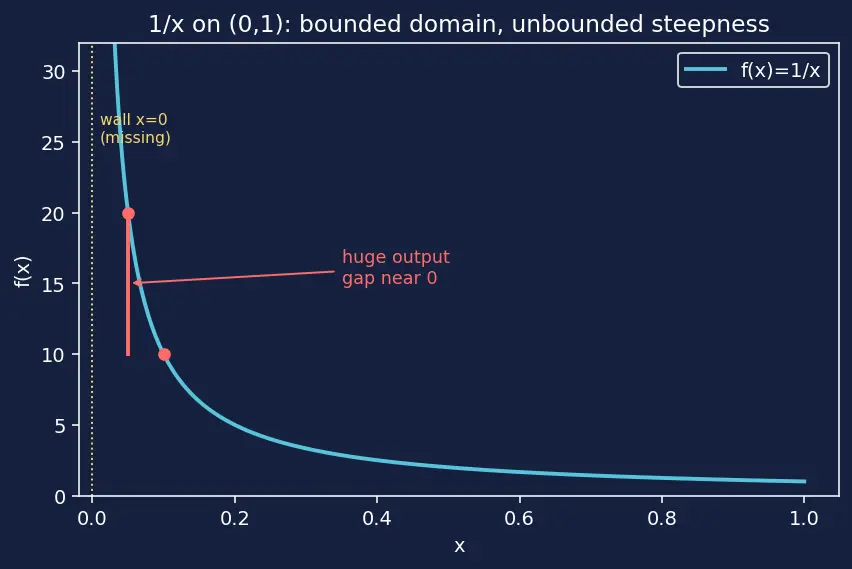
1. WHAT: note karo ki $(0,1)$ not closed hai: point $0$ missing hai, aur $f\to \infty$ as $x\to 0^{+}$. Yeh step kyun? Heine–Cantor Theorem ko closed AND bounded (Compactness) chahiye. Missing $0$ closedness todta hai, toh koi guarantee nahi — hum directly test karte hain.

2. WHAT: $\epsilon =1$ fix karo; koi bhi $\delta >0$ lo; $0$ ko hug karte points lo: $x=\delta ,y=\frac{\delta }{2}(\text{chhote }\delta \text{ ke liye dono }(0,1)\text{ mein}).$ Gap $|x-y|=\delta /2<\delta$. Dekho

   

   (figure: $1/x$ curve $x=0$ par yellow dotted wall ke approach mein upar shoot karta hai; wall ke paas ek red pair of points dikhata hai ki ek tiny sideways step ek huge vertical leap produce karta hai). Yeh step kyun? Steepness $0$ ke paas rehti hai, toh hum pair ko us wall ke against crowd karte hain.

3. WHAT: output gap measure karo. $|\frac{1}{x}-\frac{1}{y}|=|\frac{1}{\delta }-\frac{2}{\delta }|=\frac{1}{\delta }.$ $\delta <1$ ke liye yeh $>1=\epsilon$ hai. Yeh step kyun? Output gap $1/\delta \to \infty$ as $\delta \to 0$ — kisi bhi tolerance ko beat karta hai, toh koi single $\delta$ kaam nahi karta.

Verify: $\delta =0.1\Rightarrow x=0.1,y=0.05$: $|x-y|=0.05<0.1$ ✓, $|1/x-1/y|=|10-20|=10>1$ ✓.

---

Ex 4 — Cell D: non-Lipschitz lekin phir bhi uniformly continuous

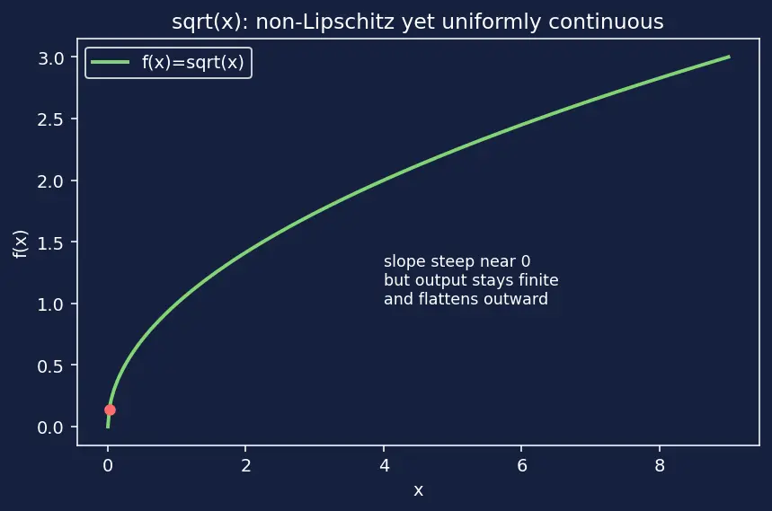
Forecast: slope $\frac{1}{2\sqrt{x}}\to \infty$ near $0$ — wahi warning sign jaise $1/x$. $\sqrt{x}$ kyun survive karta hai jahan $1/x$ mara?

1. WHAT: Lipschitz ko ek fixed $L$ chahiye hoga $|\sqrt{x}-\sqrt{y}|\le L|x-y|$ ke saath. Near $0$ derivative $f^{\prime }(x)=\frac{1}{2\sqrt{x}}\to \infty$, toh koi finite $L$ nahi exist karta. Yeh step kyun? Hum pehle maante hain ki easy test fail hota hai — Lipschitz sufficient hai, necessary nahi.

2. WHAT: square-root inequality scratch se prove karo. WLOG maano $x\ge y\ge 0$, toh $\sqrt{x}\ge \sqrt{y}\ge 0$. $(\sqrt{x}-\sqrt{y}{)}^2$ ko $x-y=(\sqrt{x}-\sqrt{y})(\sqrt{x}+\sqrt{y})$ se compare karo: $(\sqrt{x}-\sqrt{y}{)}^2=(\sqrt{x}-\sqrt{y})(\sqrt{x}-\sqrt{y})\le (\sqrt{x}-\sqrt{y})(\sqrt{x}+\sqrt{y})=x-y,$ kyunki $\sqrt{x}-\sqrt{y}\le \sqrt{x}+\sqrt{y}$ (humne sirf non-negative $2\sqrt{y}$ doosre factor mein add kiya jabki pehla factor $\sqrt{x}-\sqrt{y}\ge 0$ hai). $(\sqrt{x}-\sqrt{y}{)}^2\le |x-y|$ ke square roots lete hue milta hai $|\sqrt{x}-\sqrt{y}|\le \sqrt{|x-y|}.$ Yeh step kyun? Yeh poore example ka engine hai, toh hum ise derive karte hain quote karne ki bajaye: chhote factor $(\sqrt{x}-\sqrt{y})$ ko bade $(\sqrt{x}+\sqrt{y})$ se replace karne se product sirf increase ho sakta hai, aur woh bada product exactly $x-y$ hai.

3. WHAT: growth padhо. Output gap sirf $\sqrt{\text{input gap}}$ ki tarah grow karta hai — ek gentler growth. $1/x$ ke unlike, function bounded aur finite rehta hai har jagah, $0$ pe bhi; iska graph flattern hota hai (steep nahi) jaise $x$ grow karta hai.

   

   mein mild slope compare karo (figure: green $\sqrt{x}$ curve origin se steeply rise karke flatten hoti hai; $0$ ke paas ek red dot mark karta hai jahan slope sabse bada hai, phir bhi output finite rehta hai).

4. WHAT: $\delta ={\epsilon }^2$ choose karo. Tab $|x-y|<{\epsilon }^2⟹|\sqrt{x}-\sqrt{y}|\le \sqrt{|x-y|}<\sqrt{{\epsilon }^2}=\epsilon .$ Yeh step kyun? $\delta$ sirf $\epsilon$ pe depend karta hai — Lipschitz ke bina uniformity achieve ho gayi.

Verify: $\epsilon =0.1\Rightarrow \delta =0.01$. Worst near-$0$ pair $x=0.01,y=0$: $|x-y|=0.01=\delta$ (boundary), $|\sqrt{x}-\sqrt{y}|=0.1$, jo $\le \epsilon$ hai. ✓

---

Ex 5 — Cell E: Mean Value Theorem se Lipschitz constant hunt karo

Forecast: $\sin$ forever wiggle karta hai — kya "forever" uniformity ko $x^2$ ki tarah break karta hai?

1. WHAT: derivative compute karo aur usse bound karo. $f^{\prime }(x)=\cos x$, aur $|\cos x|\le 1$ sabhi $x$ ke liye. Yeh step kyun? ek bounded slope Lipschitz ka sabse clean route hai. Yahan $L=1$ — poori line ke liye ek single number.

2. WHAT: Mean Value Theorem invoke karo. Kisi bhi $x,y$ ke liye unke beech ek $c$ exist karta hai $\sin x-\sin y=\cos c(x-y)\Rightarrow |\sin x-\sin y|=|\cos c||x-y|\le 1\cdot |x-y|.$ Yeh step kyun? MVT "bounded derivative" ko "bounded output-to-input ratio" mein convert karta hai, yani $L=1$ ke saath Lipschitz.

3. WHAT: $\delta =\epsilon$ choose karo (kyunki $\delta =\epsilon /L=\epsilon /1$). $|x-y|<\epsilon ⟹|\sin x-\sin y|\le |x-y|<\epsilon .$ Yeh step kyun? $\delta$ mein koi $x$ nahi — uniform, even though graph oscillate karna band nahi karta. Wiggle height aur steepness mein bounded hai, $x^2$ ki ever-growing steepness ke unlike.

Verify: $\epsilon =0.05\Rightarrow \delta =0.05$. $x=0,y=0.05$ lo: $|\sin x-\sin y|=|\sin 0.05|=0.049979<0.05$ ✓.

---

Ex 6 — Cell F: bounded oscillation jo PHIR BHI fail karti hai

Forecast: output kabhi $[-1,1]$ nahi chhoda — toh output gaps $\epsilon$ se kaise exceed kar sakte hain?

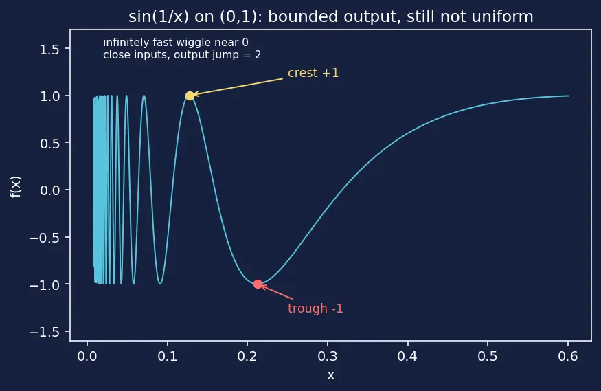
1. WHAT: $\epsilon =1$ fix karo; koi bhi $\delta >0$ lo. $0$ ke paas wiggle ke do peaks/valleys choose karo, ek positive integer $n$ se indexed: $x_n=\frac{1}{2\pi n+\frac{\pi }{2}},y_n=\frac{1}{2\pi n-\frac{\pi }{2}}.$ Tab $f(x_n)=\sin (2\pi n+\frac{\pi }{2})=1$ aur $f(y_n)=\sin (2\pi n-\frac{\pi }{2})=-1$. Yeh step kyun? $0$ ke paas graph infinitely fast oscillate karta hai, toh ek $+1$ crest aur ek $-1$ trough arbitrarily close saath baithte hain — dekho

   

   (figure: blue $\sin (1/x)$ curve $0$ ki taraf tezi se aur tezi se wiggle karta hai; ek yellow dot ek $+1$ crest mark karta hai aur ek red dot ek nearby $-1$ trough mark karta hai, toh do close inputs ka output jump $2$ hai).

2. WHAT: domain membership check karo. Har integer $n\ge 1$ ke liye denominators satisfy karte hain $2\pi n-\frac{\pi }{2}>2\pi \cdot 1-\frac{\pi }{2}=\frac{3\pi }{2}>1$, toh dono $x_n,y_n\in (0,\frac{2}{3\pi })\subset (0,1)$. Har $n\ge 1$ legal hai; koi smallness assumption zaroorat nahi. Yeh step kyun? Hume confirm karna hoga ki engineered points actually domain mein rehte hain unhe use karne se pehle, aur yahan even $n=1$ safely $(0,1)$ ke andar land karta hai.

3. WHAT: sideways gap estimate karo taaki kisi bhi $\delta$ ko beat kar sakein. Do fractions ko common denominator pe subtract karke, $|x_n-y_n|=\left|\frac{1}{2\pi n+\frac{\pi }{2}}-\frac{1}{2\pi n-\frac{\pi }{2}}\right|=\frac{\pi }{\left(2\pi n+\frac{\pi }{2}\right)\left(2\pi n-\frac{\pi }{2}\right)}=\frac{\pi }{(2\pi n{)}^2-{\left(\frac{\pi }{2}\right)}^2}\underset{n\to \infty }{\to }0.$ Toh kisi bhi $\delta >0$ ke liye, itna bada $n$ choose karo ki yeh quantity $<\delta$ ho; dono points step 2 se $(0,1)$ mein rehte hain. Yeh step kyun? Explicit formula $\frac{\pi }{(2\pi n{)}^2-(\pi /2{)}^2}$ prove karta hai ki crests $0$ pe bunch up hoti hain — hum sirf assert nahi karte.

4. WHAT: phir bhi output gap hai $|f(x_n)-f(y_n)|=|1-(-1)|=2>1=\epsilon .$ Yeh step kyun? Bounded output tumhe nahi bachata — jo matter karta hai woh yeh hai ki close inputs ab bhi ek fixed jump of $2$ de sakte hain. Frequency, amplitude nahi, uniformity ko kill karta hai.

Verify (n=1): $x_1=1/(2\pi +\pi /2)\approx 0.1273$, $y_1=1/(2\pi -\pi /2)\approx 0.1819$; $|x_1-y_1|\approx 0.0546<0.1$, output gap $=2>1$ ✓.

---

Ex 7 — Cell G: limiting/boundary repair UC restore karta hai

Forecast: kya ek single missing point plug karna ek "maybe" ko guaranteed UC mein turn kar sakta hai — aur kya hum phir bhi ek concrete closeness rule likh sakte hain?

1. WHAT: open end pe limit compute karo. ${\lim }_{x\to 0^{+}}\frac{\sin x}{x}=1.$ Yeh step kyun? Compactness ko rokne wali sirf yeh cheez thi ki missing endpoint $0$ tha. Agar function ka wahan finite limit hai, toh hum hole ko continuously fill kar sakte hain.

2. WHAT: $g(0)=1$ set karo. Ab $g$ closed bounded interval $[0,1]$ pe continuous hai. Yeh step kyun? $[0,1]$ compact hai; Ex 3 ke open $(0,1)$ ke unlike, kuch bhi infinity ki taraf nahi jaata.

3. WHAT (qualitative): Heine–Cantor Theorem apply karo: compact set pe continuous $\Rightarrow$ uniformly continuous. Yeh step kyun? Humne ek boundary defect ko ek compact domain mein convert kar diya, aur theorem baaki kar deta hai.

4. WHAT (quantitative $\delta$): hum $\delta$ haath se banate hain, aur slope bound ko assert karne ki bajaye prove karte hain. Likho $g^{\prime }(x)=\frac{x\cos x-\sin x}{x^2}$ $x>0$ ke liye (aur $g^{\prime }(0)=0$ symmetry se, kyunki $g$ even hai). $x\in (0,1]$ ke liye valid do standard inequalities use karo: $\sin x\ge x-\frac{x^3}{6},\cos x\le 1.$ Tab numerator satisfy karta hai $x\cos x-\sin x\le x\cdot 1-(x-\frac{x^3}{6})=\frac{x^3}{6},$ aur ($\sin x\le x$, $\cos x\ge 1-\frac{x^2}{2}$ use karte hue) yeh bhi satisfy karta hai $x\cos x-\sin x\ge x(1-\frac{x^2}{2})-x=-\frac{x^3}{2}$. Hence $|g^{\prime }(x)|=\frac{|x\cos x-\sin x|}{x^2}\le \frac{\max (\frac{x^3}{6},\frac{x^3}{2})}{x^2}=\frac{x}{2}\le \frac{1}{2}\text{for }x\in (0,1].$ Toh $|g^{\prime }|\le \frac{1}{2}$ poore $[0,1]$ pe. Mean Value Theorem se yeh Lipschitz constant $L=\frac{1}{2}$ deta hai, toh $\delta =\frac{\epsilon }{L}=2\epsilon ,|x-y|<2\epsilon \Rightarrow |g(x)-g(y)|\le \frac{1}{2}|x-y|<\epsilon .$ Yeh step kyun? Heine–Cantor ek $\delta$ guarantee karta hai; Taylor-type bounds $\sin x\ge x-\frac{x^3}{6}$ aur $\cos x\ge 1-\frac{x^2}{2}$ "one checks" ko ek genuine everywhere-valid inequality $|g^{\prime }|\le \frac{x}{2}\le \frac{1}{2}$ mein turn karte hain, jo humein ek explicit $\delta$ deta hai.

Verify: limit numerically: $\sin (0.001)/0.001=0.99999983\approx 1$ ✓; aur bound: $[0,1]$ pe $|g^{\prime }|$ ka actual maximum $x=1$ pe hai, $|g^{\prime }(1)|\approx 0.30\le \frac{1}{2}$, hamare proven bound $|g^{\prime }(x)|\le x/2$ ke consistent ✓, toh $L=\frac{1}{2}$ ek safe (loose) Lipschitz constant hai.

---

Ex 8 — Cell H: real-world word problem

Forecast: kya ek closeness rule poore run ko cover karta hai, ya yeh time ke saath change karna padega?

1. WHAT: steepest rate of change find karo (derivative bound karo). $T^{\prime }(t)=3-\frac{1}{5}t,|T^{\prime }(t)|\le \max (|T^{\prime }(0)|,|T^{\prime }(10)|)=\max (3,1)=3\frac{{}^{\circ }\text{C}}{\text{min}}.$ Yeh step kyun? Compact interval $[0,10]$ pe bounded slope $L=3$ Mean Value Theorem se Lipschitz deta hai — "one rule everywhere" ka physical version.

2. WHAT: Lipschitz bound: $|T(s)-T(t)|\le 3|s-t|$. Yeh step kyun? "Temperature kitni fast move kar sakti hai" ko "do readings kitni door ho sakti hain" mein turn karta hai.

3. WHAT: $3\delta =\epsilon$ solve karo: $\delta =\frac{\epsilon }{L}=\frac{0.5}{3}\approx 0.1667$ minutes ($\approx 10$ seconds). Yeh step kyun? $\delta$ sirf tolerance aur slope bound pe depend karta hai — kis minute hum sample karte hain us pe nahi. Uniformity = poori shift ke liye ek compliance rule.

Verify: worst case near $t=0$ (steepest): $T(0)=20$, $T(0.1667)=20+0.5-0.00278=20.497$; gap $=0.497<0.5$ ✓. Units: $\frac{{}^{\circ }\text{C}}{\text{min}}\times \text{min}={}^{\circ }\text{C}$ ✓.

---

Ex 9 — Cell I: products pe exam twist

Forecast: yeh tempting lagta hai ki "do well-behaved functions ka product bhi well-behaved hoga." Padhne se pehle haan ya na bet karo — exam trap yeh hai ki answer no hai.

1. WHAT: derivative ko growing slope ke liye test karo. $f^{\prime }(x)=\sin x+x\cos x,|f^{\prime }(x)|\ge |x\cos x|-|\sin x|.$ $x=2\pi n$ pe: $\cos (2\pi n)=1,\sin (2\pi n)=0$, toh $f^{\prime }(2\pi n)=2\pi n\to \infty$. Yeh step kyun? Unbounded slope classic warning flag hai (recall $x^2$). Factor $x$ oscillation ki steepness ko bina limit ke amplify karta hai — toh hum failure suspect karte hain aur bad pairs hunt karne jaate hain.

2. WHAT: sideways-close, output-far pairs engineer karo. $x_n=2\pi n$ ke near (jahan $\sin =0$, toh $f(x_n)=0$) ek nearby point $y_n=2\pi n+h$ lo jisme ek fixed chhota $h$ ho: $f(y_n)=(2\pi n+h)\sin (2\pi n+h)=(2\pi n+h)\sin h.$ Sideways gap hai $|x_n-y_n|=h$; $h<\delta$ choose karo toh yeh legally close hai. Tab $|f(y_n)-f(x_n)|=(2\pi n+h)|\sin h|\ge 2\pi n|\sin h|\underset{n\to \infty }{\to }\infty .$ Yeh step kyun? $h$ fixed hone ke saath sideways gap kabhi nahi badalta, lekin $2\pi n|\sin h|$ $n\to \infty$ ke saath without bound grow karta hai — yeh exact negation pattern Ex 2 se hai.

3. WHAT: conclude karo. Kisi bhi candidate $\delta >0$ ke liye $h=\min (\delta /2,1)$ lo (toh $h<\delta$ aur $\sin h\ne 0$), phir itna bada $n$ lo ki $2\pi n|\sin h|>\epsilon$. $\delta$ se closer aur output gap $\epsilon$ se upar wali do points exist karti hain ⇒ $x\sin x$ $\mathbb{R}$ pe nahi hai uniformly continuous. Koi rescuing $\delta (\epsilon )$ nahi hai. Yeh step kyun? Moral: uniform continuity unbounded domains pe multiplication ke under closed nahi hai — ek genuine exam trap. (Kisi bhi bounded $[a,b]$ pe yeh fine hai, Heine–Cantor se.)

Verify: $h=0.1$, $n=100$ lo toh $x=200\pi \approx 628.3185$, $y=x+0.1$: $|x-y|=0.1$, aur $|f(x)-f(y)|=|0-(628.4185)\sin (628.4185)|\approx 62.75\gg \epsilon$. $n$ double karne se yeh gap roughly double hota hai ⇒ unbounded ✓.

---

Recall Kisi bhi function pe run karne ke liye scenario checklist

Compact domain? → UC free (Heine–Cantor). Bounded derivative? → Lipschitz, $\delta =\epsilon /L$. Slope $\to \infty$ ya domain unbounded / blow-up pe open? → bad pairs hunt karo (unhe steep jagah crowd karo). Bounded output lekin infinite oscillation? → phir bhi fail ho sakta hai (Ex 6). Finite limit ke saath missing endpoint? → fill karo aur compactness gain karo (Ex 7).

Connections

• Continuity (pointwise) — woh weaker property jahan se har example start hota hai.
• Heine–Cantor Theorem — Ex 1 aur Ex 7 ko power karta hai.
• Compactness / Lebesgue number lemma — kyun closed+bounded rescue karta hai.
• Lipschitz continuity — Ex 5, Ex 8 (aur Ex 4 dikhata hai ki yeh necessary nahi hai).
• Mean Value Theorem — bounded slope → Lipschitz, Ex 5, Ex 7 & Ex 8 mein use hota hai.
• Cauchy sequences — UC Cauchyness preserve karta hai, woh deeper reason ki $1/x$ $(0,1)$ pe fail karta hai.