In the expansion ∇θlogPθ(τ), the trajectory probability factorizes into three kinds of terms: the initial-state distribution ρ(s0), the environment dynamics P(st+1∣st,at), and the policy πθ(at∣st). Which term(s) survive the gradient, and why?
Recall Solution
WHAT survives: only ∑t∇θlogπθ(at∣st).
WHY:log turns the product into a sum: logPθ(τ)=logρ(s0)+∑tlogP(st+1∣st,at)+∑tlogπθ(at∣st). The gradient ∇θ asks "how does this change when I wiggle the knobs θ?" The initial distribution and the dynamics belong to the environment — they contain no θ — so their slope is 0. Only the policy carries θ.
Consequence: we never need a model of the world → policy gradients are model-free.
A two-action softmax policy has πθ(a1)=σ(θ) and πθ(a2)=1−σ(θ). You sample a1 and receive return R=+2. With learning rate α=0.5 and current θ=0, compute the update Δθ=α∇θlogπθ(a1)R.
Recall Solution
Step 1 — the log-prob gradient.logπθ(a1)=logσ(θ). A standard identity: dθdlogσ(θ)=1−σ(θ). Why?σ′=σ(1−σ), and dθdlogσ=σσ′=1−σ.
Step 2 — plug in θ=0.σ(0)=1+e01=0.5, so ∇θlogπθ(a1)=1−0.5=0.5.
Step 3 — assemble.Δθ=α⋅0.5⋅R=0.5⋅0.5⋅2=0.5.
What it looks like:θ rises → σ(θ) rises above 0.5 → action a1 becomes more probable. A rewarded action was reinforced. ✓
An episode with γ=0.9 has rewards r0=1,r1=0,r2=2,r3=−1. Compute the reward-to-go G1=∑t′≥1γt′−1rt′.
Recall Solution
WHAT we do: sum rewards from t=1 onward, each discounted by how far in the future it is relative to t=1.
G1=γ0r1+γ1r2+γ2r3=1(0)+0.9(2)+0.81(−1)=0+1.8−0.81=0.99.WHY start the exponent at 0: the reward att=1 is "now" from t=1's viewpoint, so it gets γ0=1. r0 is excluded because an action at t=1 cannot affect the past (causality).
Show that for any function b(s) that does not depend on the action, Ea∼πθ(⋅∣s)[∇θlogπθ(a∣s)b(s)]=0.
Recall Solution
Step 1 — write the expectation as a sum over actions (discrete case):
Ea[∇θlogπθ(a∣s)b(s)]=∑aπθ(a∣s)∇θlogπθ(a∣s)b(s).Step 2 — undo the log-derivative trick. Since π∇logπ=ππ∇π=∇π:
=b(s)∑a∇θπθ(a∣s)=b(s)∇θ=1a∑πθ(a∣s).Step 3 — probabilities sum to 1, and the gradient of a constant is 0:
=b(s)∇θ1=b(s)⋅0=0.■WHY b(s) came out front: it does not depend on a, so it is a constant with respect to the sum over a. That is the whole reason a state-only baseline is allowed but an action-dependent one is not.
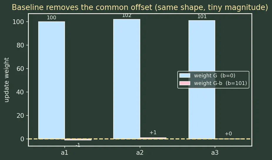
Given three actions with returns G∈{100,102,101}, compare the spread of the update weights with baseline b=0 versus b=Gˉ=101. What does this say about variance?
Recall Solution
The update weight on each action is (G−b).
b=0: weights {100,102,101}, mean 101, spread around a huge common offset.
b=101: weights {−1,+1,0} — the offset is removed; only the differences that matter remain.
WHY variance drops: the Monte-Carlo estimator's variance scales with the magnitude of these weights (roughly E[(G−b)2∥∇logπ∥2]). With b=0 every weight is ∼100, so sampling noise on ∇logπ gets amplified 100×. Subtracting Gˉ centers the weights near zero without changing the expected gradient (Q3.1), so we keep the signal and kill the amplified noise.
The figure shows the same three weights before (tall bars far from zero) and after (short bars straddling zero) subtracting the baseline — same shape, dramatically smaller magnitude.
In a state s you have three actions whose sampled reward-to-go values are G(a1)=8,G(a2)=2,G(a3)=5, each sampled once with equal policy probability. Estimate V(s) as the mean return, then compute the advantage A(s,a)=G(a)−V(s) for each action. Which actions get reinforced, which get suppressed?
Recall Solution
Step 1 — baseline V(s): the natural estimate is the average return, V(s)=38+2+5=5.
Step 2 — advantages:A(s,a1)=8−5=+3,A(s,a2)=2−5=−3,A(s,a3)=5−5=0.Step 3 — interpretation via the update θ+=α∇logπ⋅A:
a1: A>0 → pushed up (better than average).
a2: A<0 → pushed down (worse than average).
a3: A=0 → no change (exactly average).
WHY this is the seed of Actor-Critic methods: replace the hand-averaged V(s) with a learned critic Vϕ(s), and you turn REINFORCE-with-baseline into actor-critic. The advantage A is the shared currency; see Advantage function and Generalized Advantage Estimation.
Suppose a plain REINFORCE estimate has variance s2 per trajectory and you average N independent trajectories. If a baseline reduces per-trajectory variance to s2/9, how many un-baselined trajectories N′ would you need to match the accuracy of N=20 baselined trajectories?
Recall Solution
Step 1 — accuracy = variance of the average. For N i.i.d. samples the mean's variance is (per-sample variance)/N.
Baselined, N=20: variance =20s2/9=180s2.
Un-baselined, N′: variance =N′s2.
Step 2 — match them:N′s2=180s2⇒N′=180.
Answer:N′=180 un-baselined trajectories — 9× more data for the same accuracy. This is the practical payoff of Variance reduction in Monte Carlo.
A softmax policy over two actions uses logits z1=θ,z2=0, so
πθ(a1)=eθ+e0eθ=σ(θ),πθ(a2)=1−σ(θ).
Start at θ=0. You run one episode: sample a1, and the environment returns G=+2 for this action (baseline b=0). Then run a second episode: sample a2, return G=+2 as well, still b=0.
(a) Compute ∇θlogπθ(a2) symbolically.
(b) Give both updates with α=1, then the net θ after both (apply sequentially, recomputing σ).
(c) Explain what goes wrong here and how a baseline of b=2 fixes it.
Recall Solution
(a) Gradient of the losing branch.logπθ(a2)=log(1−σ(θ)). Since dθd(1−σ)=−σ(1−σ),
∇θlogπθ(a2)=1−σ−σ(1−σ)=−σ(θ).
(Compare Q2.1's ∇θlogπθ(a1)=+(1−σ) — the two branches have opposite-signed gradients, as they must, since raising one lowers the other.)
(b) Sequential updates (α=1, b=0).
Episode 1 at θ0=0, σ=0.5: sampled a1, weight G=2.
Δθ=1⋅(1−σ)⋅2=1⋅0.5⋅2=+1.0. New θ1=1.0.
Episode 2 at θ1=1.0, σ(1)=1+e−11≈0.7311: sampled a2, weight G=2.
Δθ=1⋅(−σ)⋅2=1⋅(−0.7311)⋅2≈−1.4621. New θ2≈1.0−1.4621=−0.4621.
(c) What went wrong.Both actions gave the same return +2, so neither is genuinely better — yet we still shoved θ around by more than a full unit each step. With b=0, every positive return is treated as "reinforce me," so the updates are dominated by the common offset, not by real differences. The net wandered to −0.46 purely from ordering/noise, not from any signal.
The baseline fix. Set b=2. Now each weight is G−b=0, so both updates are exactly 0: θ stays put at 0. That is the correct behavior — when two actions are equally good, the policy should not move. The baseline stripped the meaningless common offset, leaving only the (here, zero) advantage. This is exactly Q3.1's unbiasedness paying off as Q3.2's variance reduction.