Attention visualization and limitations: Exercises

These problems build from reading an attention matrix to reasoning about why it can mislead you. Every symbol used here is built in the parent note and in Attention Mechanisms. Work each one before opening the solution.

Reminders of the two objects we compute with:

$A = softmax (\frac{Q K ^{T}}{d _{k}}), A_{ij} \geq 0, \sum_{j} A_{ij} = 1$

The row $A_{i, :}$ is a probability distribution: it says where query position $i$ looks. That row-sums-to-one fact is the workhorse of almost every problem below.

Level 1 — Recognition

Exercise 1.1 — Read a single row

An attention matrix over tokens ["The", "cat", "sat"] has query-row for "sat" equal to $A_{sat, :} = [0.1, 0.7, 0.2] .$ (a) Which token does "sat" attend to most? (b) What must $0.1 + 0.7 + 0.2$ equal, and why?

Recall Solution

(a) The largest entry is $0.7$ , in the "cat" column, so "sat" attends most to =="cat"==. (b) The entries must sum to $0.1 + 0.7 + 0.2 = 1.0$ . Why: each row is a softmax output — softmax exponentiates then divides by the total, so a row is a probability distribution that always sums to $1$ .

Exercise 1.2 — Softmax by hand

Two raw attention scores (pre-softmax) are $s = [2, 0]$ . Compute the attention weights.

Recall Solution

Softmax exponentiates each score then normalizes: $e^{2} = 7.389, e^{0} = 1.$ Sum $= 8.389$ . Weights: $[\frac{7.389}{8.389}, \frac{1}{8.389}] = [0.881, 0.119] .$ The bigger score gets the bigger share, but the small one is never zero — softmax gives strictly positive weights.

Level 2 — Application

Exercise 2.1 — Scaling changes the sharpness

Query $q = [1, 1]$ , keys $k_{1} = [1, 1]$ , $k_{2} = [1, - 1]$ , dimension $d_{k} = 2$ . Compute the two attention weights with the $d_{k}$ scaling.

Recall Solution

Dot products: $q \cdot k_{1} = 1 + 1 = 2$ , $q \cdot k_{2} = 1 - 1 = 0$ . Scale by $d_{k} = 2 \approx 1.414$ : scores $= [2/1.414, 0] = [1.414, 0]$ . Softmax: $e^{1.414} = 4.113$ , $e^{0} = 1$ , sum $= 5.113$ . $[0.804, 0.196] .$ Why the scaling? Without dividing by $d_{k}$ the score would be $2$ giving $[0.881, 0.119]$ (Exercise 1.2) — sharper. Scaling flattens the distribution so gradients through softmax don't vanish in high dimensions.

Exercise 2.2 — Averaging heads

Three heads give the "it"→"animal" weight as $0.9, 0.1, 0.2$ . Compute the mean-attention value $\overset{ˉ}{A}$ .

Recall Solution

$\overset{ˉ}{A} = \frac{0.9 + 0.1 + 0.2}{3} = \frac{1.2}{3} = 0.4.$ Note how one confident head ( $0.9$ ) got diluted to $0.4$ by two quiet heads.

Level 3 — Analysis

Exercise 3.1 — Attention rollout, two layers

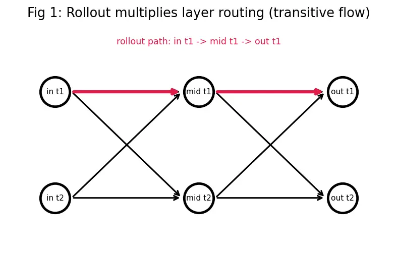
Two single-head layers, no residual term, over 2 tokens: $A^{(1)} = [0.8 0.3 0.2 0.7], A^{(2)} = [0.5 0.1 0.5 0.9] .$ Compute the rollout $A_{roll} = A^{(2)} A^{(1)}$ and read off how much token 1's output depends on input token 1.

Recall Solution

Matrix product $A^{(2)} A^{(1)}$ :

Row 1: $[0.5 (0.8) + 0.5 (0.3), 0.5 (0.2) + 0.5 (0.7)] = [0.55, 0.45]$
Row 2: $[0.1 (0.8) + 0.9 (0.3), 0.1 (0.2) + 0.9 (0.7)] = [0.35, 0.65]$ $A_{roll} = [0.55 0.35 0.45 0.65] .$ Entry $(1, 1) = 0.55$ : why the product? Layer 1 routes input $\to$ mid, layer 2 routes mid $\to$ output. The product's $(i, j)$ entry sums over the intermediate token $k$ : $\sum_{k} A_{ik}^{(2)} A_{k j}^{(1)}$ — the transitive information path. See figure

Exercise 3.2 — Rollout with identity (residual)

Same $A^{(1)}$ as above. Form $\tilde{A}^{(1)} = A^{(1)} + I$ , then row-normalize it (this is the residual-stream trick from the parent note).

Recall Solution

$A^{(1)} + I = [1.8 0.3 0.2 1.7] .$ Row sums: $2.0$ and $2.0$ . Divide each row by its sum: $\tilde{A}_{norm} = [0.9 0.15 0.1 0.85] .$ Why add $I$ ? The residual connection copies each token's own value straight through, so a token attends partly to itself. Adding $I$ then renormalizing bakes that self-pass into the routing matrix, keeping rows summing to $1$ .

Level 4 — Synthesis

Exercise 4.1 — Attention high, contribution zero

Token $j$ gets attention $α_{ij} = 0.9$ but its value vector is $v_{j} = [3, 3]$ and the downstream layer projects onto direction $w = [1, - 1]$ (its sensitivity). Compute the effective contribution $α_{ij} (v_{j} \cdot w)$ and interpret.

Recall Solution

$v_{j} \cdot w = 3 (1) + 3 (- 1) = 0$ . $Contribution = 0.9 \times 0 = 0.$ Despite $0.9$ attention, this token contributes nothing: its value vector lies in the null space of the downstream direction. This is the headline limitation — attention weight measured the look, not the effect. See figure

Figure — Attention visualization and limitations

Exercise 4.2 — Attention vs gradient disagreement

For output $y$ and two tokens, attention weights are $[0.8, 0.2]$ but loss gradients are $\frac{\partial L}{\partial x _{1}} = 0.05, \frac{\partial L}{\partial x _{2}} = 0.9$ . Rank the tokens by attention and by gradient. What does the disagreement tell you?

Recall Solution

By attention: token 1 ( $0.8$ ) $>$ token 2 ( $0.2$ ). By gradient: token 2 ( $0.9$ ) $>$ token 1 ( $0.05$ ). They disagree. Token 1 was looked at heavily but changing it barely moves the loss (examined, not used). Token 2 was barely attended but the loss is very sensitive to it (indirect influence). Attention shows correlation; the gradient shows causation — see SHAP for Deep Learning and Probing Classifiers for causal probes.

Level 5 — Mastery

Exercise 5.1 — Design an adversarial attention pair

You have output $o = \sum_{j} α_{j} v_{j}$ with values $v_{1} = [1, 0]$ , $v_{2} = [1, 0]$ , $v_{3} = [0, 5]$ and original weights $α = [0.5, 0.5, 0]$ . Find a different weight vector $α^{'}$ (a valid distribution) that produces the same output $o$ , demonstrating attention is not identifiable.

Recall Solution

Original output: $o = 0.5 [1, 0] + 0.5 [1, 0] + 0 [0, 5] = [1, 0]$ . Since $v_{1} = v_{2}$ , any split between positions 1 and 2 keeps position 3 at weight $0$ gives the same $o$ . Choose $α^{'} = [0.9, 0.1, 0] .$ Check: $0.9 [1, 0] + 0.1 [1, 0] + 0 [0, 5] = [1, 0] = o .$ ✓ Meaning: two visibly different heatmaps ( $[0.5, 0.5, 0]$ vs $[0.9, 0.1, 0]$ ) produce an identical result. When value vectors are duplicated (or degenerate), attention weights are not uniquely determined — the core Jain–Wallace critique, formalized. See figure

Exercise 5.2 — Full contribution pipeline

Combine everything. Token $j$ : $α_{ij} = 0.6$ , $v_{j} = [4, 3]$ , downstream sensitivity direction $w = [0, 1]$ (unit vector). Compute (a) $∥ v_{j} ∥$ , (b) the aligned magnitude $∣ v_{j} \cdot w ∣$ , (c) the effective contribution $α_{ij} ∣ v_{j} \cdot w ∣$ , and compare against the naive "attention only" score $α_{ij}$ .

Recall Solution

(a) $∥ v_{j} ∥ = 4^{2} + 3^{2} = 25 = 5$ . (b) $v_{j} \cdot w = 4 (0) + 3 (1) = 3$ , so $∣ v_{j} \cdot w ∣ = 3$ . (c) Contribution $= 0.6 \times 3 = 1.8$ . Naive attention score would report $0.6$ . The true routed magnitude is $1.8$ — nearly triple, because this value vector is both large and well-aligned with what the next layer reads. Attention alone under-reported this token. Lesson: always fold in $∥ v_{j} ∥$ and alignment, never rank by $α$ in isolation.

Recall Self-test cloze

Attention rows always sum to ::: $1$ (they are softmax / probability distributions) Attention shows correlation, gradients show ::: causation Two attention maps can give the same output when value vectors are ::: duplicated or degenerate (non-identifiability) True contribution $\approx α_{ij}$ times ::: $∥ v_{j} ∥$ times downstream sensitivity

Related tools: BertViz Tool for interactive heatmaps · Transformer Architecture for where these matrices come from · Hinglish version.