First momentmt = EMA of the gradient: mt=β1mt−1+(1−β1)gt. It smooths the direction — this is the momentum idea.
Second momentvt = EMA of the squared gradient: vt=β2vt−1+(1−β2)gt2. It smooths the magnitude — this is the RMSProp idea.
One tracker says where to go, the other says how big a step is safe there.
Recall Solution
(P) is AdamW. The decay term −ηλθt−1 sits outside the v^t fraction, so it is never divided by the magnitude tracker. See Weight Decay and L2 Regularization.
(Q) is Adam+L2. The λθt−1 is folded into gt, so it flows through mt,vt and gets divided by v^t — the very bug AdamW removes.
Recall Solution
It is a signal-to-noise ratio. m^t is the mean gradient, v^t is its typical size.
Ratio ≈1: the gradient points consistently the same way (mean ≈ magnitude) ⇒ confident, take a full step of size ≈η.
Ratio ≈0: the gradient jitters around zero (mean ≪ magnitude) ⇒ unsure, take a tiny step.
This is a form of variance-aware stepping.
step =0.01⋅0.5/0.25=0.01⋅0.5/0.5=0.01, so θ2=0.99−0.01=0.98.
On a constant gradient the corrected estimates stay pinned at m^=g, v^=g2, so every step keeps size η. This is the steady-state behaviour previewed in the parent note.
Recall Solution
The decay part is −ηλθt−1, so θ←θ(1−ηλ).
Surviving fraction =1−ηλ=1−0.001⋅0.1=1−0.0001=0.9999.
Each step shrinks every weight by 0.01% — the same for all weights, which is exactly what classical weight decay wants.
At t=1: m1=(1−β1)g1 and v1=(1−β2)g12.
Bias correction: m^1=1−β1(1−β1)g1=g1, and v^1=1−β2(1−β2)g12=g12.
Step =ηv^1m^1=ηg12g1=η∣g1∣g1=ηsign(g1).
The magnitude is ∣ηsign(g1)∣=η, free of ∣g1∣. Look at figure s01: the SGD step (yellow) grows with the gradient, while the Adam step (blue) is clamped to length η in both cases.
Figure s01 caption: horizontal axis = gradient magnitude ∣g∣; vertical axis = step magnitude. Yellow line = SGD step η∣g∣ (a straight line through the origin, growing without bound). Blue flat line = Adam's first step =η (constant at height η=1 regardless of ∣g∣). Dotted markers at ∣g∣=0.5 and ∣g∣=2.5 show SGD leaping to different heights while Adam stays pinned.
Recall Solution
Replace gi→cgi for all i. Both EMAs are linear in their inputs:
mt→cmt (since m is a weighted sum of gradients), so m^t→cm^t.
vt→c2vt (inputs are gi2→c2gi2), so v^t→c2v^t, hence v^t→cv^t.
Step =ηcv^tcm^t=ηv^tm^t — the c cancels.
Consequence: Adam is immune to global gradient rescaling (e.g. a change of loss units). Plain SGD is not — its step ηcg scales with c.
Recall Solution
With ϵ=0: step =η10−1010−4=η10−510−4=10η — a 10× blow-up.
With ϵ=10−8: v^t+ϵ=10−5+10−8≈1.001×10⁻⁵, step ≈η1.001×10−510−4≈9.99η. Barely different here.
Now push v^t→0: with ϵ=0 the step →∞; with ϵ the step is capped at ηm^t/ϵ. So ϵ is not just anti-divide-by-zero — it bounds the maximum effective learning rate in near-flat regions. It is a real hyperparameter.
Decay contribution = the part of the step coming from the λθ term.
(i) Adam+L2: the λθ is folded into the gradient, so it is divided by v^:
decay=ηv^λθ.
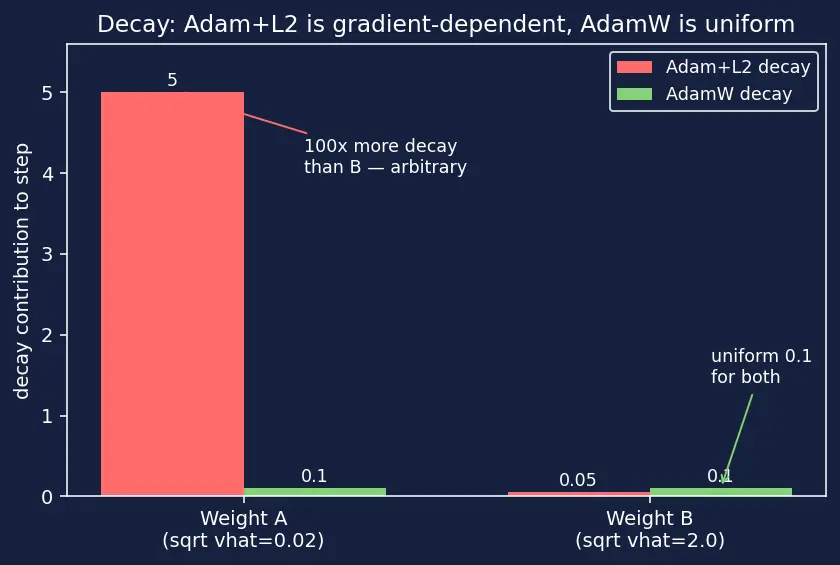
A: 1⋅0.020.05⋅2=0.020.1=5.0.
B: 1⋅2.00.05⋅2=2.00.1=0.05.
A is decayed 100× harder than B — purely because of gradient history. Backwards.
(ii) AdamW:decay=ηλθ=1⋅0.05⋅2=0.1 for bothA and B.
Uniform, gradient-independent — the correct behaviour. Figure s02 shows the two decay bars.
Figure s02 caption: grouped bar chart. Left group = weight A, right group = weight B. Red bars = Adam+L2 decay contribution (5.0 for A, 0.05 for B — a 100× spread). Green bars = AdamW decay contribution (0.1 for both — equal height). The visual punch: red bars are wildly uneven, green bars are identical, showing AdamW's uniform shrinkage.
Recall Solution
Unroll the EMA from m0=0:
mt=(1−β1)∑i=1tβ1t−igi.
Take expectations, using E[gi]=gˉ:
E[mt]=gˉ(1−β1)∑i=1tβ1t−i.
The sum is a geometric series ∑k=0t−1β1k=1−β11−β1t. So
E[mt]=gˉ(1−β1)⋅1−β11−β1t=gˉ(1−β1t).
This is smaller than the target gˉ by the factor (1−β1t). Dividing mt by that factor gives E[m^t]=gˉ — unbiased. As t→∞, β1t→0 and the correction →1 (vanishes). The identical argument on the squared stream gives v^t=vt/(1−β2t).
Recall Solution
flowchart TD
  G["raw gradient g_t"] --> M["update m_t EMA of g"]
  G --> V["update v_t EMA of g squared"]
  M --> MH["bias correct m hat"]
  V --> VH["bias correct v hat"]
  MH --> R["ratio m hat over root v hat"]
  VH --> R
  R --> U["subtract eta times ratio"]
  TH["current weight theta"] --> D["decay subtract eta lambda theta"]
  U --> NEW["new weight"]
  D --> NEW
Node TH is the current weight θt−1; node D is the decay step −ηλθt−1 applied straight to it. The decay arrow (TH --> D) feeds the weight in directly, never touching the ratio node R. Adam+L2's mistake is to instead route decay through node G (fold λθ into the gradient), so it passes through V/VH and gets divided by v^. AdamW keeps the two paths separate.
Observable: the norm of the very first update, ∥Δθ1∥, relative to η.
Correct Adam: at t=1, per-coordinate ∣Δθ∣=η exactly (from L3-Q1). So ∥Δθ1∥/η=d for d parameters — a clean, gradient-independent value.
Bug (both corrections off): use raw m1=(1−β1)g1 and raw v1=(1−β2)g12. Per-coordinate step =η(1−β2)∣g1∣(1−β1)∣g1∣=η1−β21−β1. The ∣g1∣ cancels, giving a gradient-independent constant: 1−β21−β1=0.0010.1=0.03160.1=10≈3.162.
Signature: the buggy first-step norm is ∥Δθ1∥/η≈3.162d instead of the correct d. Concretely, dividing the measured first-step norm by ηd should give ≈1 if correct, ≈3.16 if both corrections are missing — a clean, model-size-independent tell.
Recall Solution
Pick AdamW. Mechanistic argument:
Transformer parameters have wildly different gradient scales across layers/embeddings, so a per-parameter adaptive rate (RMSProp-style v^) is worth more than a single SGD rate.
Heavy overfitting means regularization strength must be predictable. Adam+L2 makes decay gradient-dependent (L4-Q1: 100× spread between weights), so you cannot reason about how hard any weight is being pulled to zero.
AdamW's decoupled ηλθ shrinks every weight by the identical factor (1−ηλ) each step, giving clean, tunable regularization on top of the adaptive step.
Net: you get the adaptivity of Adam and honest weight decay — exactly why AdamW is the default for transformers.
Recall Solution
The AdamW decay term is −ηλθ. If η≈0 during warmup, then decay ≈0 too — regularization is effectively off while η is small, because decay is scaled by the sameη as the gradient step.
Fixes:
Use a decay strength that is applied on a schedule decoupled from η (some implementations let you scale decay by a fixed rate independent of the warmup η).
Or accept that regularization ramps in with the warmup, and set the schedule/λ so that over the full run the accumulated shrinkage ∏t(1−ηtλ) reaches the intended target. The lesson: in AdamW, η multiplies both the step and the decay, so any η-schedule silently reshapes regularization over time.
First-step Adam magnitude (any g=0) ::: exactly η
Steady-state Adam step on constant g ::: ηsign(g)
AdamW surviving fraction per step from decay ::: 1−ηλ
What multiplying all gradients by c does to the Adam step ::: nothing (scale-invariant)
The factor mt is biased low by at step t ::: (1−β1t)
The one thing decay in AdamW is NOT decoupled from ::: the learning rate η